The random transaction model

A couple of months ago, a colleague and I discussed politics, the economy, and ecology. Beyond our different perspectives, we could agree on one point: it looks like we are screwed. My friend and I are PhD students in artificial intelligence, and we are both interested in understanding underlying reasons, and maybe if, beyond our shared beliefs, we were wrong after all?

So he talked to me about some toy model coded by another friend of his. The model was so simple, and the claimed result was so striking I couldn’t believe it. It was so disturbing that I had to check it myself!

It’s your turn not to believe me:

1. Imagine a population of N agents starting with the same amount of money, let’s say 100$.
2. Next, choose randomly and uniformly two agents for a transaction: agent1 gives a fixed amount to agent2, let’s say 1$.
3. Now repeat the process over and over.

So this is it, this is the model! Now you might think: “What can you do with such a model?!” If so, this would be close to my initial reaction! Well, wait for it because first I have a question for you:

For a big enough number of iterations, what distribution of wealth would you expect in the end?

If you are familiar with the topics of data science, mathematics, or finance, your answer might be: “a bell curve!”

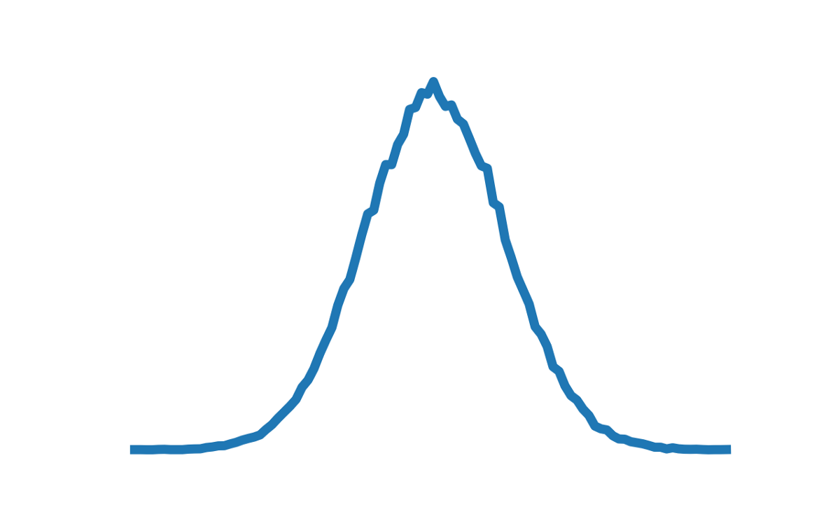
And this is logical because here, transactions are random. Some of you might recall the central limit theorem, which, by quoting Wikipedia, states: “When independent random variables are added, their […] sum tends toward a normal distribution” i.e., a bell curve.

Let’s play!

Alright, let’s start to play with this model. Assume we have 1000 agents, and all of them possess 100$ at the start.

NB: Here is a link to my code if you want to try it. You will find a lot of parameters to play with, some of which will be discussed in the following articles!

I will run 50000 iterations; 500 random transactions will occur at each iteration. For simplicity, we will have a fixed transaction amount of 1$ only. Throughout the article, no debt will be allowed, meaning that an agent will never give anything if its money is 0.

Warm-up

To forge an intuition on how this model works, we start by manually doing the first three iterations. For the sake of simplicity and without loss of generality, we will assume that in each step, the agents are randomly split into two distinct groups: the receivers and the givers. For example, at the first step, 500 agents give 1$, and the remaining 500 agents receive the given 1$, and so on:

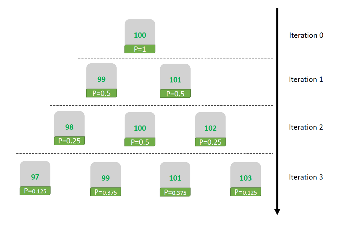
1. Iteration: the 100$ group of iteration 0 is cut in half, one half receives 1$, the other gives 1$, hence a probability P of 0.5 for both values, 99$(P=0.5) and 100$(P=0.5).
2. Iteration : both 99$ and 100$ group of iteration 1 are cut in half: 99(P=0.5) split in a group of 98(0.25) and 100(0.25); the 101(0.5) group split into 100(0.25), and 102(0.25), hence P(100)=0.25+0.25=0.5.
3. Iteration: repeat the same process!

These first three iterations drew a distribution that resembles a Gaussian distribution. Indeed it is symmetric around the average (=100$), and the probability gets higher the closer to the mean. Of course, we assumed that givers and receivers are two distinct groups, but since, in actuality, it is not, the distribution should be smoother. So these first steps seem in agreement with our mathematical intuition:

So, that’s it, problem solved. The final distribution is indeed a bell curve!

Alright, you guessed it: it is not! Otherwise, I would not have written this article in the first place.

So what is it?

Surprisingly, after the 50000 iterations, the wealth distribution looks like this :

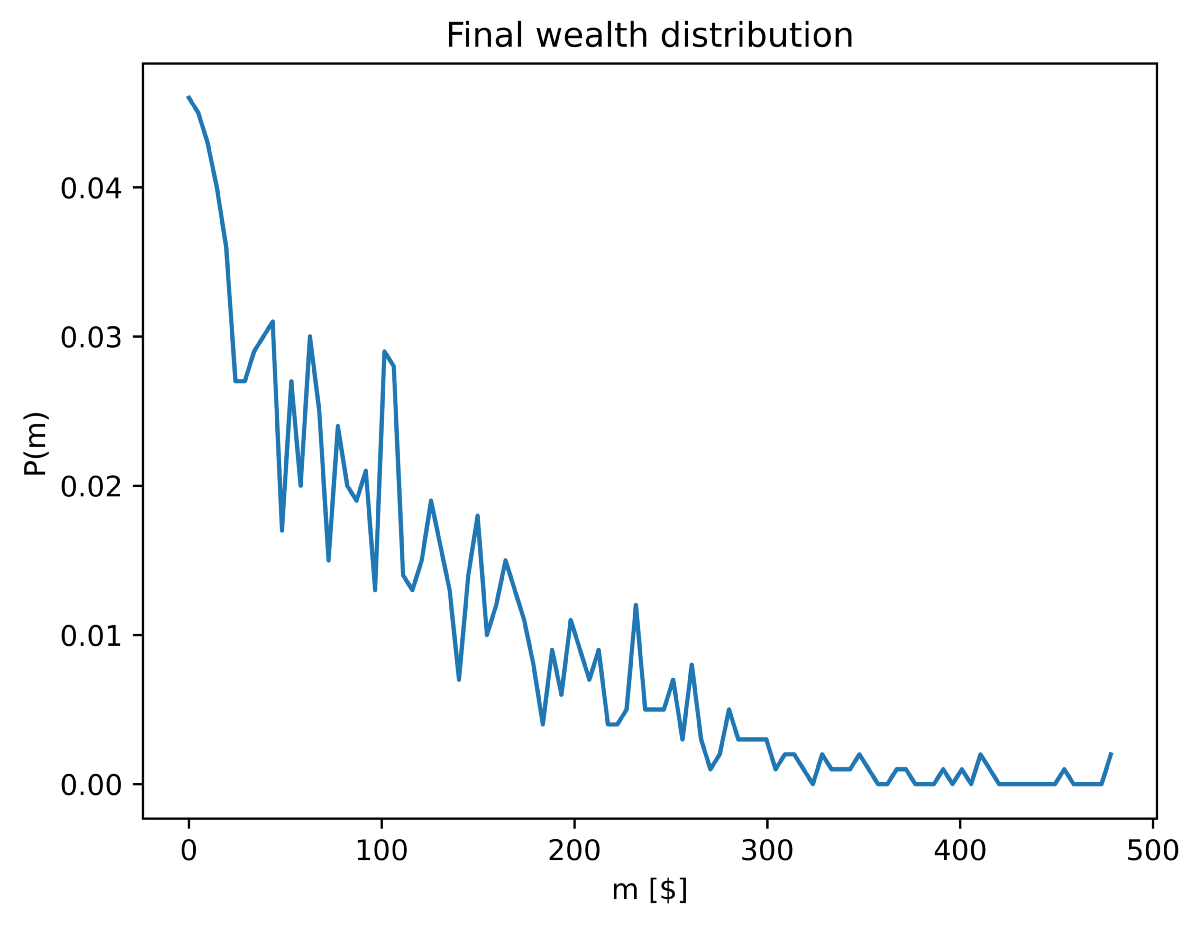
The figure shows the money probability distribution for all our 1000 agents at the last iteration. The vertical axis displays the probability P or the chance that an arbitrary agent possesses the amount of money m associated with the horizontal axis. So by looking precisely at the probabilities, the highest is obtained for m=0$, with a value P(0)~0.045, or 4.5%. As you increase the amount of money, the probability gets lower and lower and converges toward zero.

What is this distribution, might you ask: it is exponential!

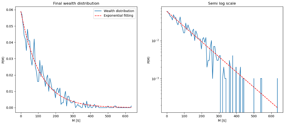
To confirm this, I displayed the curve with two representations:

1. First, you will recognize the plot on the left side, as it is the last curve in blue, with the red dotted curve representing the exponential fitting.
2. On the right side, a logarithmic scaling is applied to the vertical axis. It is equivalent to passing the probability P(m) in a 10-base logarithm, such that two numbers, for example, 1000=10³ and 100=10², will be spaced by one unit on the axis it is convenient to compress data that spans long-range values. Mathematically, applying a natural log gives a straight line:

The parameter $a$ in the equation is equal to one over the average of money possessed by all agents. By getting rid of the sign, we have $|1/a|=<~m> =106$, which is the approximated average money. This approximation from the exponential fitting is not perfect but close to the initial given value. The average is the sum of all money, divided by the number of participants. Since the total amount of money and number of agents stayed the same throughout the simulation. Whatever the shape of the initial and final distribution, we will still get the same average value. So you understand why the average is tricky to interpret.

To get a better sense of how equally the money is distributed, we can use another tool: the cumulative distribution function.

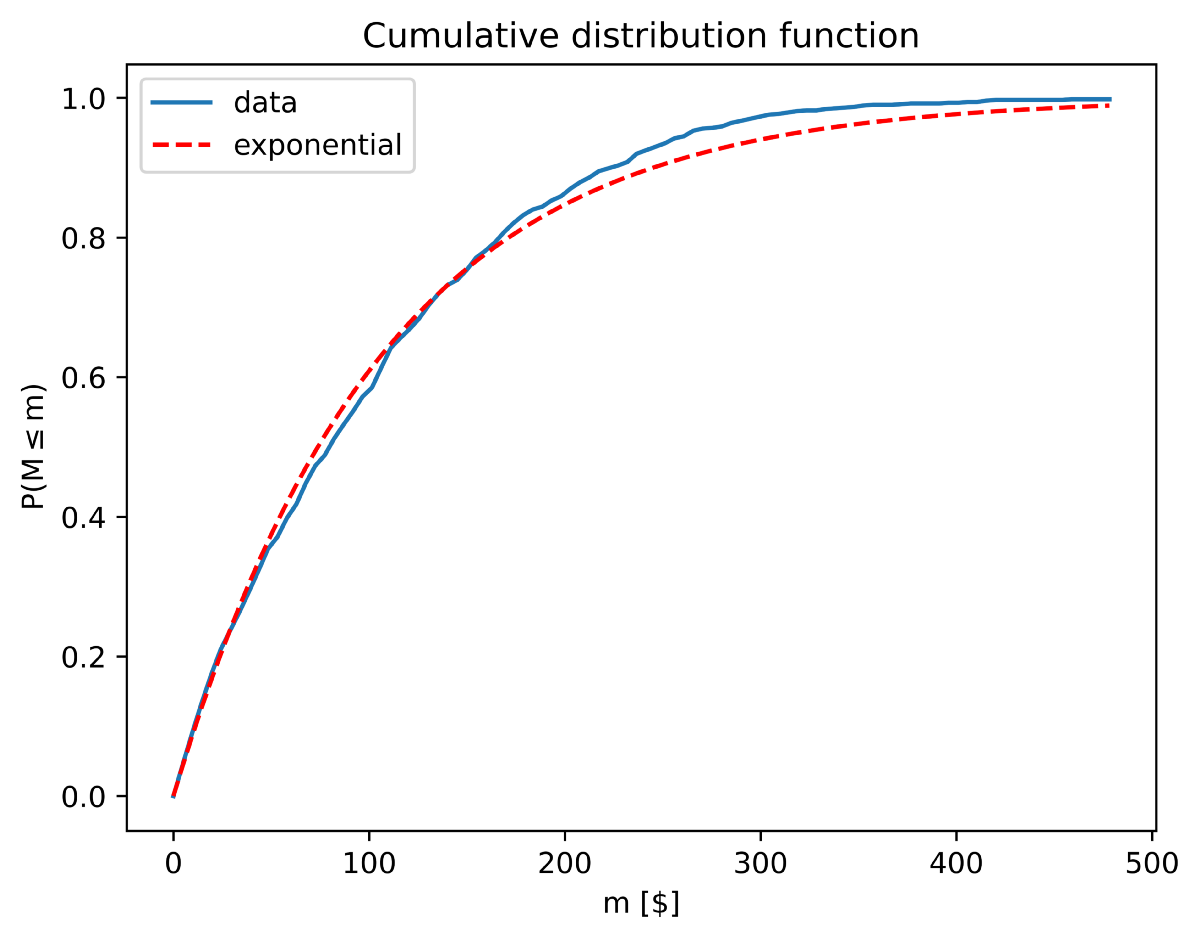
With this function, we can now ask interesting questions like:

What is the chance of having less than 200$?

The answer is straightforward: look at the corresponding point in the vertical axis, and the answer is directly P=0.8 ~80%! You might want to know how many people are under the initial amount of money, 100$, and it is around 60%! As I told you earlier, the average is indeed a bit misleading. You would be better off using the median, which precisely gives the amount of money separating the group in half: 75$. So as you see, this value is significantly lower than the average.

As a summary, if you run my code you will obtain the 80/20 separation:

There is 80.4% of people detaining 50.9% of the total wealth, and 19.6% detaining the 49.1% remaining.

How is it relevant?

We have seen a model that considered only uniform random transactions, with an equal amount of money given to every agent at the start. The model describes a very utopian society. Not only does it assume a perfectly egalitarian start. But a uniformly random exchange means there are no preferences in any specific directions, which implies a flatland of people’s attention and needs! A picture far from reality, after all, the probability that Jeff Bezos receives your money, is relatively but surely, biased in his favour! This model removes all attractors of attention: Google, Facebook, Tesla, and sorry Jeff, goodbye space travel! Finally, by saying that everyone has an equal chance of exchanging goods, we are by corollary, removing greed and avarice from the picture. But give the model sufficient time, and it ends up following an exponential distribution! This is why the final result seems very odd. It is in contradiction with our mathematical intuition and generalization capability, and we mourn already:

“Damn it, where is the bell curve?”

Okay, that’s an inevitable question, and I will try to answer it, but for that, I would need another full article! So instead, let’s go goi back to the bell curve: imagine a society with a bell curve wealth. The best way to describe it, is the paradise of the middle class. With the Gaussian distribution, the average money represents the most probable amount of money in the population. You would probably end social class clash too, since the edges of the distribution, e.g., poor and rich, would be equally unlikely events.

On the other hand, with the exponential distribution, being very poor is the baseline and the most probable state for an agent. You would have half of the population significantly below the average while being rich would be the less likely event. By observing the detailed probability distribution in the log scale, one can note that the probability of being among the richest is of the order 1/N (N being the number of agents). So the bigger the society, the harder it is to get there! In this asymmetrical reality, extreme poverty is the rule, average wealth is a chance, and being rich remains a dream. Yes, this is a fundamentally different reality from the one described by the Bell curve, and honestly, it might look familiar [2], does it?

Do we find these exponential laws in real-world data?

The answer is yes! I asked permission to show you a powerful result from this article [3]. I am sure it will speak for itself:

Conclusion

This article shows how a very simple model of uniformly random exchanges can display a very counter-intuitive result, breaking a common assumption in probability: the central limit theorem. The intuition indeed suggests that the final distribution should be Gaussian, resulting in a very fair distribution of wealth. Surprisingly, it is not! As I showed, the final distribution is exponential: an unfair distribution that is in strike contrast with the choice of a seemingly very utopian model. We chose the initial condition as an equal amount of money for all agents; we kept a very minimalist dynamic where no agents could monopolize attention, by assuming uniform random exchanges. Finally, I explained how these two distributions prescribe a very different societal reality.

However, an important question remains:

Why does this model end up with an exponential distribution?

In the following article of this series: The Physics of Economy, I will try to answer this question, and we will see how using statistical physics, this seemingly odd result suddenly becomes a “trivial” textbook exercise!

Acknowledgement

Thanks to my colleagues and friends for the review and the valuable comments. Thanks as well to the publishers for the valuable feedback and insightful questions.

References

[1] Victor Yakovenko, (2007, Augst, 22). Computer Animation of Money Exchange Models. Econophysics Research by Victor Yakovenko. Retrieved from http://www.physics.umd.edu/~yakovenk/econophysics/

[2] Max Roser and Esteban Ortiz-Ospina, (2017, March, 27). Global Extreme Poverty. Our World in Data. Retrieved from https://ourworldindata.org/extreme-poverty.

[3] Tao, Y., Wu, X., Zhou, T. et al. Exponential structure of income inequality: evidence from 67 countries. J Econ Interact Coord 14, 345–376 (2019). https://doi.org/10.1007/s11403-017-0211-6.

[3] Tao, Y., Wu, X., Zhou, T. et al. Exponential structure of income inequality: evidence from 67 countries. J Econ Interact Coord 14, 345–376 (2019). https://doi.org/10.1007/s11403-017-0211-6.