Single-qubit and multi-qubit states
Welcome to this series of labs to learn the Qiskit library for quantum computing. This series will give you the building blocks to understand quantum machine learning. You can find the code in my github repository.
This first lab will teach you how to write Qiskit code and investigate single-qubit and multi-qubit states using the Bloch-sphere and qpshere visualization. Finally, you will run a parametrized circuit on a real quantum computer!
This tutorial is adapted from Lab 1 of Qiskit courses: Introduction to Quantum Computing and Quantum Hardware.
Single-qubit states
We represent a quantum qubit state as:
\[\vert\psi\rangle = \sqrt{1-p}\vert0\rangle + e^{i\phi}\sqrt{p}\vert1\rangle\]Here, $p$ is the probability that a measurement of the state in the computational basis $( \vert0\rangle, \vert1\rangle )$ will have the outcome $1$; $\phi$ is the phase between the two computational basis states.
Single-qubit gates can be used to manipulate this quantum state by changing either $p$, $\phi$, or both.
Let’s begin by creating a single-qubit quantum circuit. We can do this in Qiskit using the following code:
from qiskit import QuantumCircuit

mycircuit = QuantumCircuit(1)
mycircuit.draw('mpl')
Output:

The above quantum circuit does not contain any gates; therefore, if you start in any state, say $\vert0\rangle$, applying this circuit to your state doesn’t change the state.
To see this clearly, let’s create the state vector $\vert0\rangle$. In Qiskit, you can do this using the following code:
from qiskit.quantum_info import Statevector

sv = Statevector.from_label('0')
You can see what’s contained in the object sv:
sv
Output:
Statevector([1.+0.j, 0.+0.j],
            dims=(2,))
A qubit vector state is a two-dimensional complex vector:
\[\LARGE \vert0\rangle = \begin{bmatrix} 1 \\0 \end{bmatrix}\]We can now apply the quantum circuit mycircuit to this state by using the evolve() method:
new_sv = sv.evolve(mycircuit)
Once again, you can look at the new statevector by writing:
new_sv
output:
Statevector([1.+0.j, 0.+0.j],
            dims=(2,))
As you can see, the state didn’t change since we didn’t add any gates yet.
Dirac notation
In the previous section, I implicitly used the Dirac notation to represent the vector state $\vert \psi\rangle$.
In a quantum mechanics textbook, you will find two essential notations associated with the way we represent vectors in the Hilbert space:
- The “ket”: is a column vector, noted $\vert \psi\rangle$.
- The “bra”: is a row vector, dual of the other, noted $\langle \psi\vert$.
When I say dual, it means that both vectors are related by a mathematical transformation that converts one into the other and vice-versa.
To be more concrete, let’s define a state vector $\vert \psi\rangle=c_1\vert1\rangle+ c_2\vert0\rangle$, with $c_1, c_2 \in \mathbb{C}$:
\[\LARGE \vert \psi\rangle= \begin{bmatrix} c_1 \\ c_2 \end{bmatrix}\]To obtain the dual, bra, we need to compute the complex conjugate transpose (denoted dagger: $\dagger$) of the ket:
\[\LARGE \vert \psi\rangle^{\dagger}= {\begin{bmatrix} c_1 \\ c_2 \end{bmatrix}}^{\dagger} = \begin{bmatrix} {c_1}^* && {c_2}^* \end{bmatrix} = \langle \psi \vert\]Okay, first, don’t be scared by the notation; this is just a different way of representing vectors. Second, as you will see in a bit, this notation makes it easy to represent states and gates as linear combination of basis vectors.
The Bloch sphere
A way to represent the state of one qubit is the Bloch sphere.
This maps the vector state $\vert\psi\rangle=\alpha\vert0\rangle+e^{i\phi}\beta\vert1\rangle$ with $\alpha, \beta \in \mathbb{R}$ to a spherical surface.
Since we have the normalization condition imposing $\sqrt{\alpha^2+\beta^2}=1$, we can first apply the trigonometry formula $\sqrt{cos(x)^2+sin(x)^2}=1$, and then use the half angle formula in order to get $\alpha$ and $\beta$ dependant of the same parameter $\theta$. Finally we get:
\[\LARGE \vert\psi\rangle=cos(\theta/2)\vert0\rangle+e^{i\phi}sin(\theta/2)\vert1\rangle\]- $\phi \in [0, 2\pi]$ describes the relative phase
- $\theta \in [0, \pi]$ describes the probability to measure $\vert0\rangle$ or $\vert1\rangle$.
We can illustrate a state on the surface of a sphere with radius $\vert\vec r\vert=1$, which we call the Bloch sphere, with a block vector of polar coordinates:
\[\LARGE \vec r = \begin{pmatrix} sin\theta \times cos\phi \\ sin\theta \times sin\phi \\ cos\theta \end{pmatrix}\]from qiskit.visualization import plot_bloch_multivector
from qiskit.quantum_info import Statevector
plot_bloch_multivector(new_sv.data)
output:
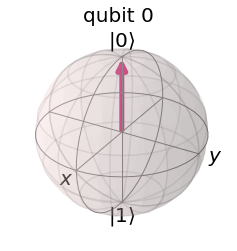
As you can see, the state $\vert0\rangle$ gets projected on the sphere’s north pole. Notice that the angle $\theta$ is divided by 2. This means that the orthogonal basis $(\vert0\rangle, \vert1\rangle)$ is stretched in the Bloch sphere, and an angle of $2\times90=180$ degree now separates each vector.
Our first gate!
Mathematically, a gate is a matrix; a single qubit matrix applies to the two-dimensional state and transforms this state into a new one; hence it’s a $2\times2$ matrix.
Here is the mathematical definition of the $X$ gate, or the quantum equivalent of the classical NOT gate:
If we apply the $X$ gate to our initial state $\vert 0\rangle$ we obtain:
\[\LARGE \sigma_x\vert 0\rangle=\begin{bmatrix}0 & 1 \\ 1 & 0 \end{bmatrix} \cdot \begin{pmatrix}1 \\ 0 \end{pmatrix}= \begin{pmatrix}0 \\ 1 \end{pmatrix}=\vert 1\rangle\]Now as I told you, we can take advantage of the Dirac notation to make calculation, as the $X$ can also be written:
\[\LARGE \sigma_x=\vert0\rangle \langle1\vert+\vert1\rangle \langle 0\vert\]Now let’s apply $\sigma_x$ to $\vert 0>$:
\[\LARGE \sigma_x\vert 0>= (\vert0\rangle \langle1\vert+\vert1\rangle \langle 0\vert)\vert0\rangle\]Since it is distributive, you can simplify:
\[\LARGE \sigma_x\vert 0>=\vert0\rangle \langle1\vert 0\rangle +\vert1\rangle \langle 0\vert 0\rangle\]Notice that $\langle . \vert .\rangle$ is just the dot product. By definition of the dot product, orthonormal vectors will give $0$, while identical vectors will give $1$:
- $\langle1\vert 0\rangle=0$
- $\langle 0\vert 0\rangle=1$
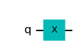
The $X$ gate flips the qubit from the state $\vert0\rangle$ to the state $\vert 1\rangle$. We will first create a single-qubit quantum circuit with the $X$ gate to see this:
mycircuit = QuantumCircuit(1)
mycircuit.x(0)

mycircuit.draw('mpl')
output:
Now, we can apply this circuit onto our state by writing:
sv = Statevector.from_label('0')
new_sv = sv.evolve(mycircuit)
new_sv
output:
Statevector([0.+0.j, 1.+0.j],
            dims=(2,))
As you can see, the statevector now corresponds to that of the state $\vert1\rangle$:
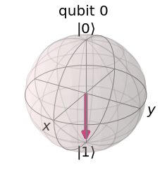
\[\LARGE \vert1\rangle = \begin{bmatrix}0\\1\end{bmatrix}\]The state can be shown on the Bloch sphere by writing:
plot_bloch_multivector(new_sv.data)
output:
Superposition
These previous states are no different from classical bits.
Now, by applying a Hadamard gate, we will create a state that is only possible in the quantum realm, a superposed state:
\[\LARGE \frac{1}{\sqrt{2}}\left(\vert 0\rangle + \vert 1\rangle\right)\]This state is a linear combination of two possible outcomes, $\vert 0\rangle$ and $\vert 1\rangle$.
To create the state, we will need the Hadamard gate, given by the following equation:
\[\LARGE H=\frac{1}{\sqrt{2}} \begin{bmatrix} 1 & 1 &\\ 1 & -1 &\\ \end{bmatrix}=\frac{1}{\sqrt{2}}\left(\vert0\rangle\langle0\vert+\vert0\rangle\langle1\vert+\vert1\rangle\langle0\vert-\vert1\rangle\langle1\vert \right)\]Here is how we can create this state and visualize it in Qiskit:
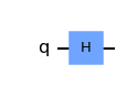
sv = Statevector.from_label('0')
mycircuit = QuantumCircuit(1)
mycircuit.h(0)
mycircuit.draw('mpl')
output:
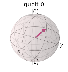
Now it’s time to plot this state on the Bloch sphere:
new_sv = sv.evolve(mycircuit)
print(new_sv)
plot_bloch_multivector(new_sv.data)
output:
Statevector([0.70710678+0.j, 0.70710678+0.j],
            dims=(2,))
As you can see above, the state is now a superposition of both basis vector $\vert0\rangle$ and $\vert1\rangle$, with an equal probability (we will compute it in the next section).
We can also create other superpositions with different phases.
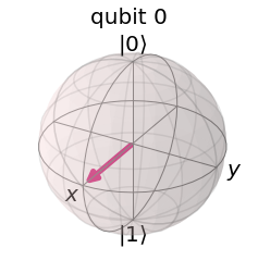
Let’s create $\frac{1}{\sqrt{2}}\left(\vert0\rangle - \vert1\rangle\right)$ which can be done by applying the Hadamard gate on the state $\vert1\rangle$.
sv = Statevector.from_label('1')
mycircuit = QuantumCircuit(1)
mycircuit.h(0)

new_sv = sv.evolve(mycircuit)
print(new_sv)
plot_bloch_multivector(new_sv.data)
output:
Statevector([ 0.70710678+0.j, -0.70710678+0.j],
            dims=(2,))
This time, the vector was rotated of the phase of $\phi = \pi$. This is because the coefficient of $\vert1\rangle$ in the state $\frac{1}{\sqrt{2}}\left(\vert0\rangle - \vert1\rangle\right)$ is $-1$, which is equal to $e^{i\pi}$.
Other phases can also be created by applying different gates. The $T$ and $S$ gates apply phases of $+\pi/4$ and $+\pi/2$, respectively. The widget below helps you see different gates, and their actions on single-qubit quantum states.
You can play around with the block-sphere : https://javafxpert.github.io/grok-bloch/)

Measuse / projection
Born Rule : the probability that a state $\vert\psi\rangle$ collpases during a projective measurement onto the state $\vert x \rangle \in \left(\vert 0 \rangle, \vert 1 \rangle \right)$ is given by :
\[\LARGE P(x) = {\left\| \langle x\vert\psi\rangle\right\|}^2\]with $\sum_i{P(x_i)=1}$.
With the previous example, the state of the qubit is:
\[\LARGE \vert \psi\rangle = \frac{1}{\sqrt{2}} (\vert 0\rangle + \vert 1\rangle)\]Let’s measure the probability of getting the qubit in the state $\vert0\rangle$ :
\[\LARGE {\left\| \langle 0\vert\psi\rangle\right\|}^2=\frac{1}{2} {\left\| \langle 0\vert(\vert0\rangle + \vert1\rangle)\right\|}^2\] \[\LARGE =\frac{1}{2} {\left\| \langle 0\vert0\rangle + \langle 0\vert1\rangle)\right\|}^2\] \[\LARGE =\frac{1}{2} {\left\| 1\right\|}^2=\frac{1}{2}\]What happens when we run the circuit?
In Quantum Computing (QC), you cannot directly get information from the qubits; you need to measure them, which will cause
a modification of their states!
- First, we use the command
QuantumCircuit(1,1)to create the circuit. The first argument asks to create a quantum circuit containing one qubit, and the second argument adds one classical bit. - Second, note that the
measurecommand takes two arguments. The first argument is the set of qubits that will be measured. The second is the set of classical bits that will store the measurement.
NB: Typically, in QC, the basis you measure is the z axis, and you cannot measure a state in superposition. You always project the qubit state with a measurable basis state $\vert0\rangle$ or $\vert1\rangle$. If ever you wanted to measure along another axis, you would have to rotate the state with the appropriate gate (for example, measurement along $x$, requires to put an $H$ gate before the measurement)
Finally, you will need to create a backend and give it to the execute function along with your circuit.
- We will use
Qiskit’s built-inqasm_simulatorbackend simulators to run the circuit. - To actually run the circuit we use the function
execute(), given a number ofshots=1000, which means the circuit will be run $1000$ times. - To get the measurement counts of these shots, we use the method
get_counts()of theresult()of thejob.
We do this by using the following code:
from qiskit import Aer, execute
from qiskit.visualization import  plot_histogram

# Create the circuit
mycircuit = QuantumCircuit(1, 1)
mycircuit.h(0)
mycircuit.measure(0, 0)

# Call a simulator backend
backend_sim = Aer.get_backend('qasm_simulator')
job = execute(mycircuit, backend_sim, shots=1000)

print(job.result().get_counts())
plot_histogram(job.result().get_counts())
output:
{'1': 493, '0': 507}
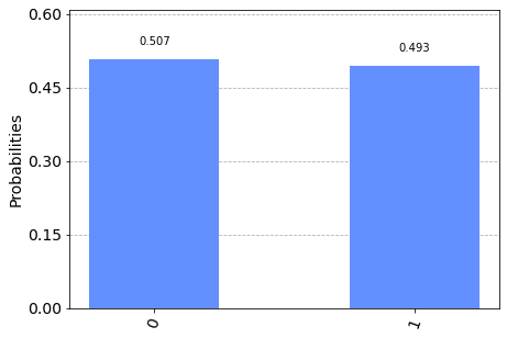
As expected each of the state is obtained close to $50\%$ of the time.
Multi-qubit states
Similar to the discussion above, you can also explore multi-qubit gates in Qiskit.
We will demonstrate below how to create the Bell state, which exploit the fundamental adventage of QC: the entanglement of qubits.
\[\LARGE \frac{1}{\sqrt{2}}\left(\vert00\rangle + \vert 11 \rangle \right)\]The state $\vert00\rangle$, means the two qubits are in the state $\vert0\rangle$ on their respective basis, and form a multi-qubit basis. You can have as many qubit as you want, such as $\vert00…0\rangle$.
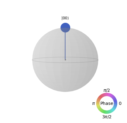
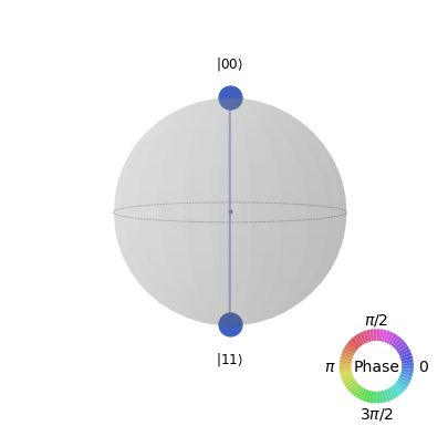
We’ll start by visualizing the state $\vert00\rangle$ using another tool, the q-sphere:
from qiskit.visualization import plot_state_qsphere

sv = Statevector.from_label('00')
plot_state_qsphere(sv.data)
output:
Next, we use the Hadamard gate described above, along with a controlled-X gate, to create the Bell state.
The controlled-X gate is an X gate that is applied if and only if the control-bit is in the $\vert1\rangle$ state. Mathematically this gives:
\[CNOT= \begin{bmatrix} 1 & 0 & 0 & 0\\ 0 & 1 & 0 & 0\\ 0 & 0 & 0 & 1\\ 0 & 0 & 1 & 0\\ \end{bmatrix}=\vert 00\rangle\langle 00\vert+\vert 01\rangle\langle 01\vert+\vert 10\rangle\langle 11\vert+\vert11\rangle\langle10\vert\]In qiskit, you can create a bell state this way:
mycircuit = QuantumCircuit(2)
mycircuit.h(0)
mycircuit.cx(0,1)
mycircuit.draw('mpl')
output:
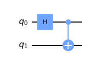
First, with the hadamard, the qubit $0$ is in a superposition of states; a linear combination $\frac{1}{\sqrt{2}}\left(\vert0\rangle + \vert1\rangle\right)$. Next, you apply a $CNOT$ on the qubit $1$, controlling it with the qubit $0$. Since the second qubit state depends on a qubit in superposition, it becomes entangled with all possible states of the first qubit!
The result of this quantum circuit on the state $\vert00\rangle$ is thus:
\[\LARGE \vert\psi^{00}\rangle=\frac{1}{\sqrt{2}}(\vert00\rangle+\vert11\rangle)\]You can display it by writing:
new_sv = sv.evolve(mycircuit)
print(new_sv)
plot_state_qsphere(new_sv.data)
output:
Statevector([0.70710678+0.j, 0.        +0.j, 0.        +0.j,
             0.70710678+0.j],
            dims=(2, 2))
As you will understand, entanglement is really one of the most important properties of quantum computing. While a classical bit can be in one state only, a quantum state with $n$ qubits can be a linear combination of $2^n$ states! In this entangled state might be hiding the solution to your problem. When performing computation, the challenge is thus to apply gates appropriately such that the system’s state is mesured to the whished solution.
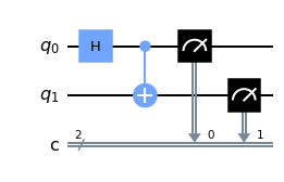
Measurements
Here is an example that creates the same Bell state and applies a measurement. In quantum mechanics, we can’t directly observe a particle in a superposition or entanglement. The only basis that we can probe is $(\vert 0\rangle, \vert 1\rangle)$. Hence measurements always project the qubits states to the $z$ axis of the Bloch sphere.
To measure we use the method mesure() and provide the indexes of first the qubits, and second the classical bits.
mycircuit = QuantumCircuit(2, 2)
mycircuit.h(0)
mycircuit.cx(0,1)
mycircuit.measure([0,1], [0,1])
mycircuit.draw('mpl')
output:
Let’s plot the histogram of counts:
from qiskit import Aer, execute
simulator = Aer.get_backend('qasm_simulator')
result = execute(mycircuit, simulator, shots=10000).result()
counts = result.get_counts(mycircuit)
plot_histogram(counts)
output:
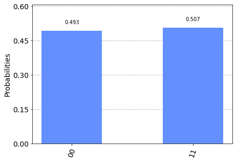
Again, the respective probability of the states is close to $0.5$.
Parametrized circuit on a real quantum computer
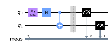
In this example, we will take the same circuit and add a Parameter. We then execute it with many values in an actual quantum circuit.
We will exploit this handy feature in the following tutorial when we have trainable parameters.
- We create a parameter $\theta$ using the class
Parameter. - We will use a gate $R_Y$, that performs rotation around the $y$ axis, parametrized by $\theta$.
- Then, we will add the bell state and measurements.
from qiskit.circuit import Parameter

theta = Parameter('theta') # Create a Parameter object
qc = QuantumCircuit(2)
qc.ry(theta, 0) # Gates can be parametrized this way
qc.h(0)
qc.cx(0, 1)
qc.measure_all()
qc.draw('mpl')
Outputs:
Now we create a list of circuit with all different initialization of the parameter:
import numpy as np

parameter_binds = {theta : 2*np.pi/3} # Dictionary
qc_a = qc.assign_parameters(parameter_binds) # A quantum circuit with given parameter

thetas = np.linspace(0, 2*np.pi, 11)
qcs = list()
for t in thetas: # You can create a list a circuit with various parameter values
    qcs.append(qc.bind_parameters({theta : t}))
Several things to note :
- We can create a list of circuits, with various initialization of parameters, and provide the list to the
execute()function. bind_parametersis a QuantumCircuit object method that allows you to bind a value to a parameter.- The arguments of this method is a
dict, of the parameter as a key, and given value as value.
- The arguments of this method is a
Connect to IBMQ
You need to log in your IBM account at the adress : https://quantum-computing.ibm.com/
Then in the first page, get your API token.
If you have trouble to connect, check to the qiskit documentation.
from qiskit import IBMQ

token = "your_token" # Replace with your token
IBMQ.save_account(token)
provider = IBMQ.load_account()
output:
ibmqfactory.load_account:WARNING:2022-03-23 15:19:31,990: Credentials are already in use. The existing account in the session will be replaced.
Now we will load a backend with a real quantum computer !
Then we will load some usefull information about this circuit.
from qiskit.visualization import plot_gate_map, plot_error_map

backend = provider.get_backend('ibmq_lima')
plot_error_map(backend)
output:
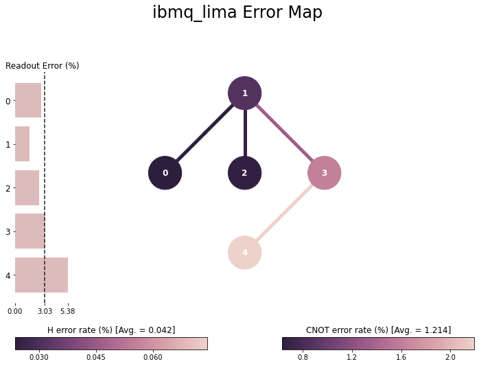
Here you can check many interesting pieces of information:
- The (%) of readout error of each qubit: You can select the qubit you want to use to minimize the error.
- The (%) of error of the
HandCNOTgate: Using too many gates can lead to high errors. - The circuit architecture: if you need to connect qubits that are not connected in the graph, you have to use
SWAPgates. They are composed of three alternatingCNOT, thus inducing even more errors!
from qiskit.tools.monitor import job_monitor

job = execute(qcs, backend, shots=1024, initial_layout=[0, 1]) # Add the two qubit you probably should use from indexes [0, 1, 2, 3 4]
job_monitor(job) # Gives status of the job
output:
Job Status: job has successfully run
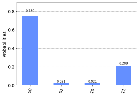
If you gave a list of several circuits to be executed, you have to give the circuit as an argument of the get_counts(), to obtain the result of the circuit you want.
import matplotlib.pyplot as plt

circ = 1 # Select the circuit you want to display
plot = plot_histogram(job.result().get_counts(qcs[circ]))
output:
Conclusion
This ends the first part of the series Hands on Quantum Computing with Qiskit. You learned how to create a quantum circuit to make simulations of superposed, and entangled qubits. And you have seen how to perform the measurement and create a parametrized circuit that can be run on a real quantum computer.
Next time we will see how to use a classical optimization of the parameters of a quantum circuit, so stay tuned!