In the previous article, I introduced the concept of elliptic curve and how it can securely produce a public key form a private key. I also proposed to explore Artificial Neural Network (ANN) as a replacement for the elliptic curve. We will design an alternative secure public key generator with the help of ANN, so let’s dive in!

I formalized the problem of generating a public key as finding a deterministic function $F$, such that:

With $F$ being not invertible, meaning that $F^{-1}$ does not exist:

Unfortunately, invertibility in a neural network is not necessarily easy to obtain. This is because, if you can train a neural network to map $y=f(x)$, in theory, you can also train another neural net to approximate the inverse $x=f’(y)$. However, we will deal with this issue in the following article.

You probably remember that we gave ourselves the challenge of not using learning in the first part. This way, we will dive into a deeper understanding of the properties of the ANN!

Designing the neural network

We are going to use a binary activation function, so let me reintroduce an image from my previous article if you need a refresher on the definition of ANN:

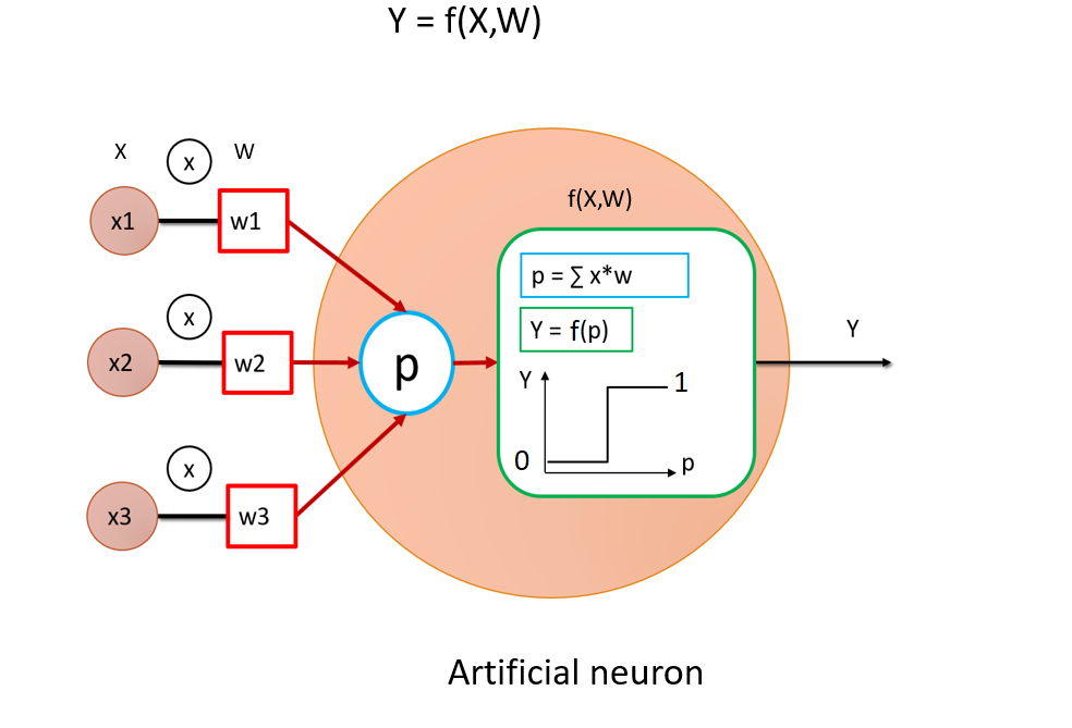
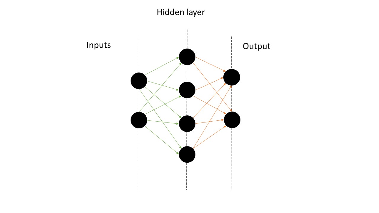
I want to design a function $F$ that takes a binary word as input and outputs a binary number. Using binary neurons is thus an obvious choice. All neuron states are either 0 or 1, depending on the sign of the weighted sum they receive in input:

One thing that is very interesting with ANN is that we can specify very easily both the size of inputs and output, such that it fits our needs, so for the rest of the article, we will choose $n=100$ bits word, both for the public and private keys. So here is the architecture of our neural network:

# Network    
inputSize = 100
outputSize = 100
hiddenSize = 100 # nb of neurons per hidden layer
nbHiddenLayer = 100
net = NeuralNetwork(inputSize, hiddenSize, outputSize, nbHiddenLayer)

For the whole article, the architecture will be constant, and we will play around with the weights of the ANN.

In the following, we assume that the network’s input and output are the vectors $X, Y \in (0, 1)^n$ with $n$ the number of bits. The output vector $Y$ of the neural network is given by:

Where $F_{net}(.)$ is the neural network function, receiving input $X$ and parametrized by parameter $W$. Note that the network itself is composed of hidden layers, each layer possessing a vector state, this will be important for the next part!

NB: I uploaded the code for the demonstration on GitHub. So I highly encourage you to check and try it by yourself.

Weight distribution

Generally, the process of finding the weights is done with machine learning technics, but here we are doing it manually because it is so much more fun, and I promise It will bring exciting insights!

So before playing with the weights, we first need a distribution; we are going to choose the normal distribution $W \sim \mathcal{N}(\mu, \sigma)$ parametrized by both its mean $\mu$ and standard deviation $\sigma$:

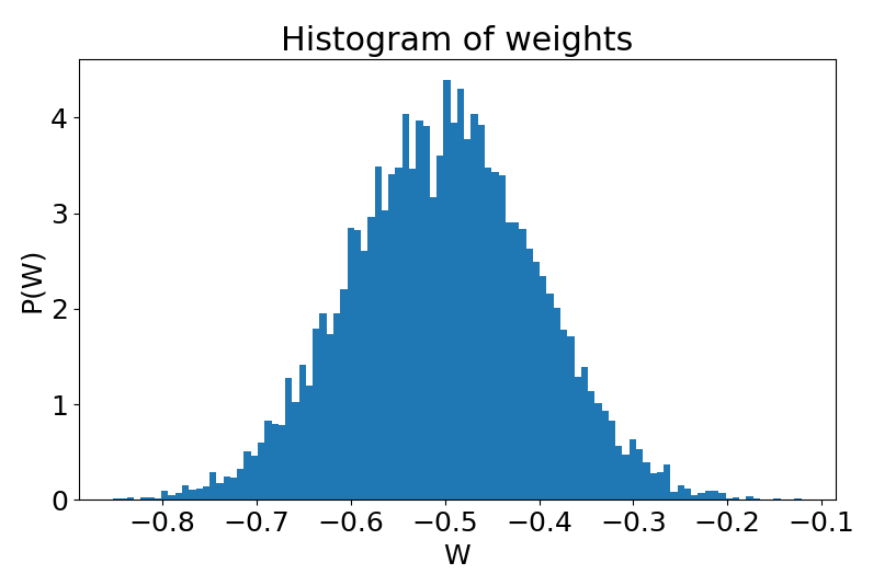
The choice of this distribution is not arbitrary, as it is a unimodal distribution, fully described by its first and second moments; higher order moments are zero. As we will see later, this is an interesting property because the output/input relationship will only be controlled by the two parameters $\mu$ and $\sigma$.

Percolation

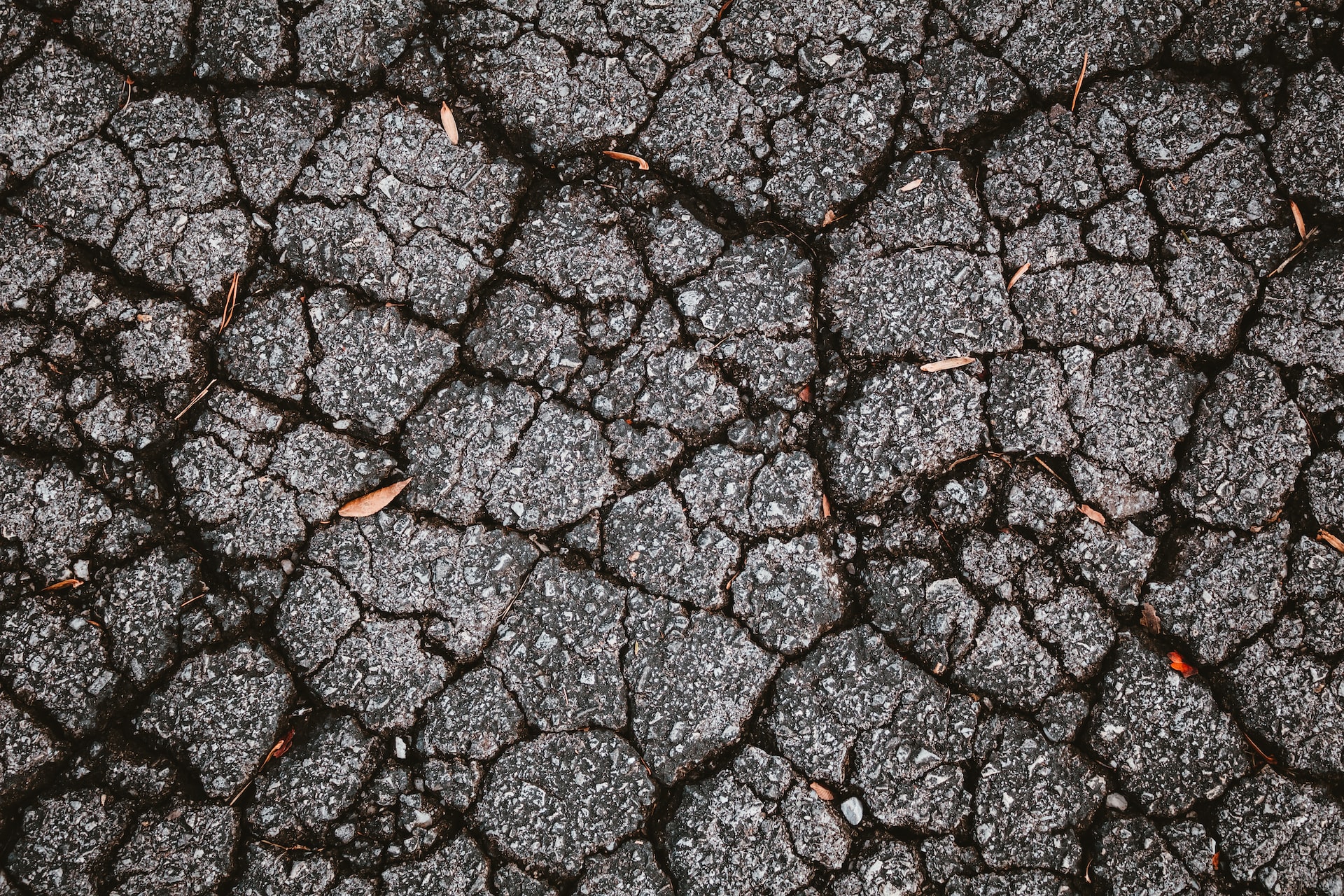
Before we can decide what parameters are the best for the weight distribution, we will build our intuition on the behaviour of this ANN. The idea here is to understand how the weights distribution parameters impact the propagation of bits, layer to layer, from the input, to the output. Now, as I will show in this section, I also chose the binary ANN because it analogous to an actual physical problem: percolation.

In physics, percolation studies the propagation of a perturbation in a substrate. For example, you can imagine someone wanting to design a physical system and evaluate water infiltration inside it. The typical percolation question could be: “How much damage before the water completely infiltrates my system?”

Stated in more general terms, this is equivalent to asking:

What is the point -in parameter space- where the perturbation traverses through the system side to side?

Now, this analogy will be evident by looking at the picture below; I plot all states of each layer as either black (0) or white (1) pixels. The horizontal axis displays the state of neurons at each layer, while the horizontal axis is the corresponding index of the layer. As such, index 0 corresponds to the input layer, which is randomly initialized, and index 101 represents the network’s output; in between, indexes represent hidden layers.

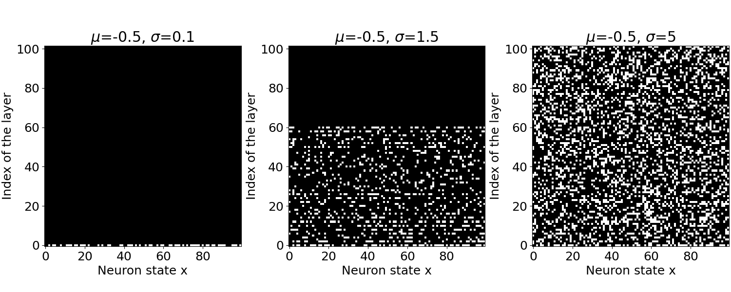
As shown in the weights histogram, the distribution for $\sigma=0.1$ only gives negative weights; thus, it is not surprising that all layers give zero states; indeed, the only way for a neuron to be active is to receive a sum of inputs greater than zero. As we increase the weight variance $\sigma=1.5$, we start to get some positive weights in the distribution, so we reach a point where the bits can propagate in the hierarchy of hidden layers. However, the bit propagation suddenly stops mid-way, and the output remains zero. This is due to the majority of inhibitory(negative) weights. Now, as we increase the variance again $\sigma=5$, the distribution has far more positive weights, and we can see that neurons in all layers are now active; this activity indeed cascades through the whole network up to the output. In that case, we reached what we call: the percolation threshold.

In theory, the percolation threshold is defined as the point in parameter space where the perturbation can propagate at infinity. Here we have $100$ layers; if our goal was to know with precision the position of this threshold, we could increase the number of hidden layers. For our purpose, $100$ is long enough since we only will transit by that point and seek out another dynamic within percolation. We will assume that the percolation threshold is reached as soon as the output is non-zero.

Now I want to stress that we are randomly generating our weight matrix and that when we reach the percolation threshold, different seeds will start giving very different results! You can observe this in the picture below, with the same parameters $\mu=-0.5$ and $\sigma=1.5$ for four other seeds.

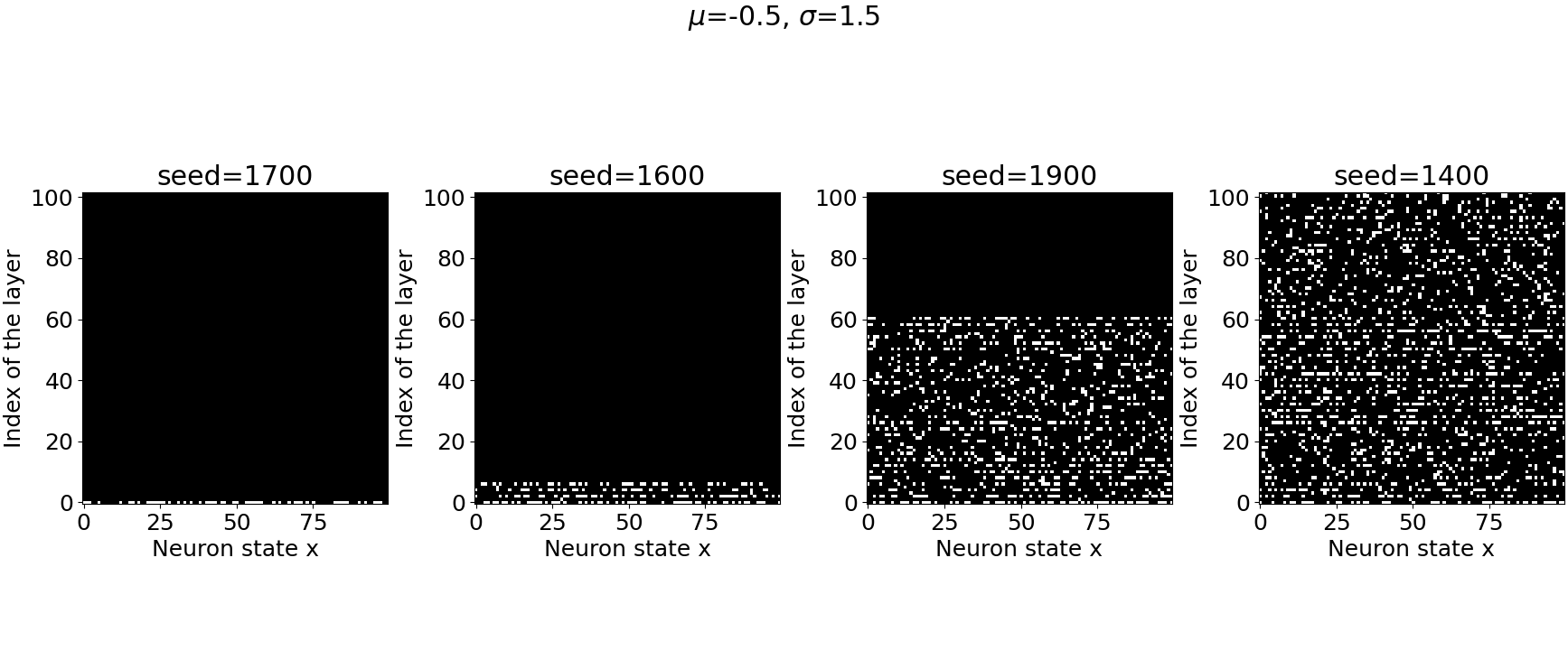
This variability in the outcomes is explained by: the sensitivity to initial condition. This is precisely what we will harness in the next part to design the $F$ function. But for now, we will draw the phase diagram, which displays the percolation transition and will reveal the best region for our parameter $\sigma$.

To illustrate the percolation transition, we can simply take the average of the output $<Y>$, obtained for different values of $\sigma$! If all output neurons are zero $<Y>=1/n\sum_i y_i$=0, the system has not percolated. On the other hand, if even one neuron is non-zero $<Y> \ne 0$, we reached the percolation threshold. Since, for some parameter regions, we saw there is some variability in the outcomes, we will average over $10$ realizations of the same weight distribution; as a result, the curve should be a bit smoother.

To generate the picture below, we took $1000$ points for $\sigma \in [0.01, 10]$. As expected, there is a parameter region where the output is always zero. The percolation threshold is exactly when the activity starts to be non-zero, so in our case with $\mu=-0.5$, it is around $\sigma_p \sim 1.4$. Above the percolation threshold, we have more and more activity in the network, and consequently, the output has more and more non-zero values; hence the averaged output increases.

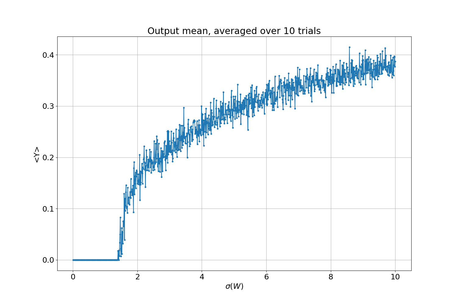
Finally, we found the region in parameter space that is of interest for our problem: it starts from the percolation threshold $\sigma_p$, for the whole non-zero output range. Now how to choose specifically in that range is not yet answered. One thing to note in that direction is that even if we averaged over ten trials, the result is still very noisy; this is because we enter a “chaotic” phase, something we will go into much more detail next part!

NB: I must insist that the step function, and for instance, any positive output activation function (so, for example, excluding the well-known sigmoid), would produce the same result. This is because a threshold needs to be crossed before any activity (state to one) can arise in the network.

Conclusion

Okay, time to wrap it up: we saw that the ANN with a step function activation is analogous to a percolation model. We have seen that by fixing the mean weight, we could play with the standard deviation of the distribution, which would be enough to control the propagation of bits through the network. We have shown that the parameter $\sigma$ controlled a phase transition from totally quiescent to highly activated. This is an interesting feature because the model here possesses $100\times100\times100=1,000,000$ parameters, which we finally reduced to one control parameter! However, sampling from the same distribution is quite noisy, and networks do not behave the same way depending on the seed we choose, which is related to the sensitivity to the initial conditions. In the following article, we will explore this in much more detail, as this is related to chaos theory, which is exactly what we need to accomplish our objective!